import jax
import jax.numpy as jnp
import matplotlib.pyplot as plt

from reactix import (
    Advection,
    Cells,
    Dispersion,
    FixedConcentrationBoundary,
    System,
    make_solver,
    declare_species,
    KineticReaction,
    reaction,
)

# Enable 64-bit floating-point precision in JAX
# See here: https://docs.kidger.site/diffrax/usage/how-to-choose-a-solver/#stiff-problems
jax.config.update("jax_enable_x64", True)Conservative tracer and first-order decay
Example model
This notebook demonstrates how to set up and run a simple reactive transport model with Reactix. The model includes two chemical species – one conservative tracer and one compound that undergoes first-order decay.
Define the species in the system
The first step is to create a list of all species in the model with declare_species. This will create a Species object where the attributes are the different chemical species. This object can be used to hold to define properties or concentrations for each species in a structured way. Next, we will use it to indicate for each species if it is transported.
Species = declare_species(["tracer", "reactive_tracer"])
species_is_mobile = Species(tracer=True, reactive_tracer=True)
Define the reactions
To set up the reactive system, we first need to define a class for each distinct reaction. In the class, we provide the rate law (in this case, first order decay) through the rate method and the corresponding coefficients as attributes of the class. In the stoichiometry method, we indicate to which species the reaction rate applies, and with which stoichiometric coefficient.
@reaction
class FirstOrderDecay(KineticReaction):
    decay_coefficient: jax.Array

    def rate(self, time, state, system):
        return self.decay_coefficient * state.reactive_tracer

    def stoichiometry(self, time, state, system):
        return {
            "reactive_tracer": -1,
        }
The value of the kinetic parameter is provided when we create an instance of the reaction class.
reactions = [FirstOrderDecay(decay_coefficient=1 / 500)]Set up the discretization
Next, we define the geometry of the cells. In this case, we create 200 equally spaced cells. The interface areas can be all equal or vary in size.
n_cells = 200
interface_areas = jnp.ones(n_cells + 1)
# interface_areas = interface_areas.at[100:].set(2) # Make one interface area larger
cells = Cells.equally_spaced(10, n_cells, interface_area=interface_areas)
Define advection and dispersion parameters and setting
The Advection and Dispersion objects hold parameters and setting needed to compute the advective and dispersive fluxes. Note that the discharge will be saved in the System object (not in Advection) because it needs to be accessed by both Advection and Dispersion (in order to compute the hydrodynamic dispersivity). The advective flow velocity is computed internally from the discharge based on the cross-sectional areas of the cells and the porosity.
dispersion = Dispersion.build(
    cells=cells,
    dispersivity=jnp.array(0.1),
    pore_diffusion=Species(
        tracer=jnp.array(1e-9 * 3600 * 24),
        reactive_tracer=jnp.array(1e-9 * 3600 * 24),
    ),
)
advection = Advection.build(
    limiter_type="minmod",
)
Define the boundary conditions
The code below shows how fixed-concentration boundaries can be set up for the different species.
Each boundary condition needs to declare which of the two boundaries and which species it will be applied to. Selecting the species work with a selector function that takes a Species object as input and returns the species of interest. The fixed concentration can be either a constant value, or it can vary with time. In the latter case, it must be specified with a function that takes time as an input and returns the corresponding boundary concentration.
If no boundary condition is specified for a species on a boundary this results implicitly in a no-flux condition.
bcs = [
    FixedConcentrationBoundary(
        boundary="left",
        species_selector=lambda s: s.tracer,
        fixed_concentration=lambda t: jnp.array(10.0),
    ),
    FixedConcentrationBoundary(
        boundary="right",
        species_selector=lambda s: s.tracer,
        fixed_concentration=lambda t: jnp.array(3.0),
    ),
    FixedConcentrationBoundary(
        boundary="left",
        species_selector=lambda s: s.reactive_tracer,
        fixed_concentration=lambda t: jnp.array(10.0),
    ),
    FixedConcentrationBoundary(
        boundary="right",
        species_selector=lambda s: s.reactive_tracer,
        fixed_concentration=lambda t: jnp.array(3.0),
    ),
]
Set up the system
The next step is to create a System object that contains all the previous settings.
porosity = jnp.ones(n_cells) * 0.3
porosity = porosity.at[100:].set(0.1)
system = System.build(
    porosity=porosity,
    discharge=lambda t: jnp.array(1 / 365) * 0.3,
    cells=cells,
    advection=advection,
    dispersion=dispersion,
    species_is_mobile=species_is_mobile,
    bcs=bcs,
    reactions=reactions,
)
Configure the solver
Next, we set solver options: the end time of the simulation, the times when a solution should be returned, and tolerances.
t_points = jnp.linspace(0, 8000, 123)
solver = make_solver(t_max=8000, t_points=t_points, rtol=1e-3, atol=1e-3)
Define initial conditions
The initial conditions must be provided as a Species object. For each species, it contains an array of concentrations (one for each cell).
# Create an array of zeros with the length of the number of cells
val0 = jnp.zeros(cells.n_cells)
# val0 = val0.at[slice(10,20)].set(10.0)

# Set up the initial conditions (all zeros in this case)
state = Species(tracer=val0, reactive_tracer=val0)
Run the solver
Finally, we run the solver to obtain the solution of the system of equations.
The output is a Solution object that contains the simulation results but also statistics on the solver run (e.g., number of steps). The attributes ys contains the output states as a Species object. It contains an array of size (n_times, n_cells) with concentrations for each species. The attribute ts of solution holds the corresponding times.
solution = solver(state, system)
# %timeit solution = solver(state, system)solution.ys.tracer.shape(123, 200)Plot the results
The following plots show the concentrations of the conservative and reactive tracer over space at different times.
You can see how the conservative tracer travels through the domain until it reaches the inflow concentration everywhere.
plt.plot(cells.centers[:], solution.ys.tracer.T[:, 0::10])
plt.title("Conservative tracer")
plt.ylabel("concentration")
plt.xlabel("x")
plt.show()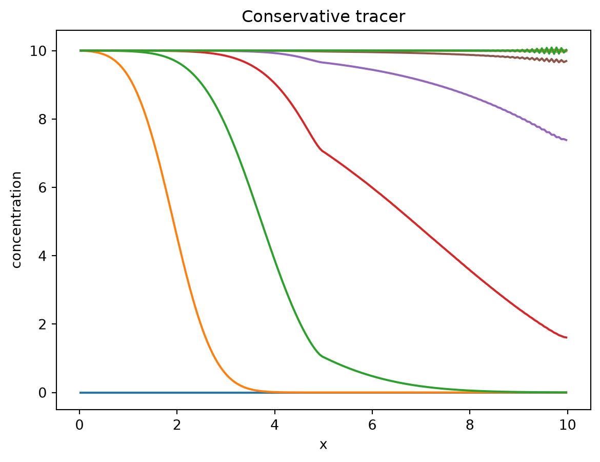
The reactive tracer initially also travels through the domain but then reaches a constant profile that is shaped by the first-order decay.
plt.plot(cells.centers[:], solution.ys.reactive_tracer.T[:, 0::10])
plt.title("Reactive compound")
plt.ylabel("concentration")
plt.xlabel("x")
plt.show()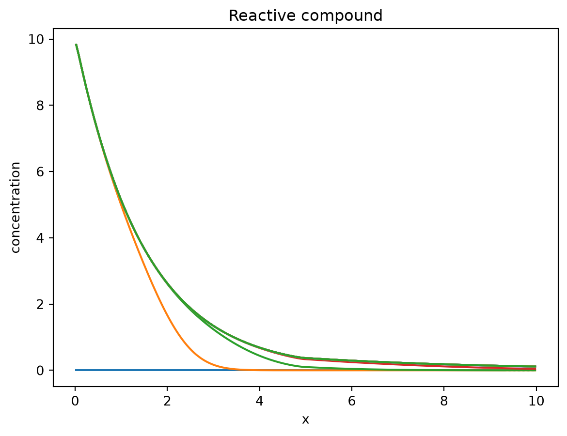
The following plot animates the two concentration profiles over time.
from IPython.display import HTML
import matplotlib.pyplot as plt
from matplotlib import animation, collections

collections.Collection()
fig, ax = plt.subplots()

artists = []
for data in zip(solution.ys.tracer, solution.ys.reactive_tracer, strict=True):
    containers = [ax.plot(cells.centers, y, color=f"C{i}") for i, y in enumerate(data)]
    artist = []
    for container in containers:
        artist.extend(container)
    artists.append(artist)


ani = animation.ArtistAnimation(fig=fig, artists=artists, interval=40)
plt.close()
HTML(ani.to_jshtml())Check the mass balance
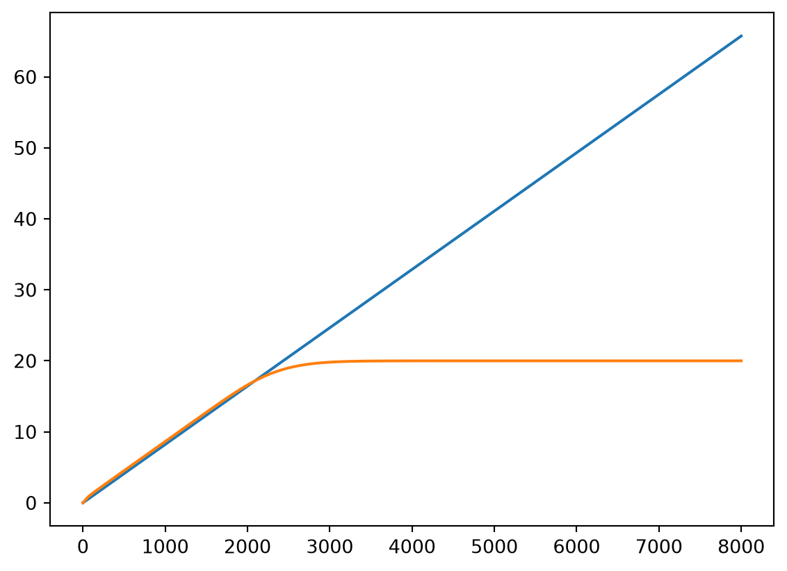
The following plot shows the mass of the conservative tracer present in the system over time, comparing it to the mass that entered the system. Up to the moment that the tracer reaches the outlet, they should be the same.
mass_in = (
    system.discharge(solution.ts)
    * bcs[0].fixed_concentration(solution.ts)
    * solution.ts
)
mass_in_system = (
    solution.ys.tracer * cells.cell_area * cells.face_distances * system.porosity
).sum(axis=1)

plt.plot(solution.ts, mass_in)
plt.plot(solution.ts, mass_in_system)
plt.show()