import jax
import jax.numpy as jnp
import matplotlib.pyplot as plt
from reactix import (
    System, Cells, Advection, Dispersion,
    FixedConcentrationBoundary, declare_species, make_solver
)Quickstart
This guide will walk you through the basics of using Reactix to set up and solve reactive transport problems.
Basic Concepts
A reactive transport model in Reactix consists three main components:
- Transport processes: Advection and dispersion of chemical species
- Chemical reactions: Kinetic reactions that transform species
- Boundary conditions: Fixed concentrations or fluxes at domain boundaries
Your First Model
Let’s build a simple 1-D transport model with a conservative tracer:
Step 1: Import Reactix
Step 2: Declare chemical species
# Define the species in your system
Species = declare_species(["tracer"])

# Specify which species are mobile (can be transported)
species_is_mobile = Species(tracer=True)
Step 3: Set up the domain geometry and transport parameters
# Create a 1-D domain with 100 cells over 10 length units
n_cells = 100
cells = Cells.equally_spaced(length=10.0, n_cells=n_cells)

# Define transport properties
advection = Advection.build(limiter_type="upwind")
dispersion = Dispersion.build(
    cells=cells,
    dispersivity=jnp.array(0.1),  # Longitudinal dispersivity
    pore_diffusion=Species(tracer=jnp.array(1e-9))  # Molecular diffusion
)
Step 4: Set boundary conditions
# Fixed concentration at inlet (left) and outlet (right)
boundary_conditions = [
    FixedConcentrationBoundary(
        boundary="left",
        species_selector=lambda s: s.tracer,
        fixed_concentration=lambda t: jnp.array(1.0)  # Constant injection
    ),
    FixedConcentrationBoundary(
        boundary="right",
        species_selector=lambda s: s.tracer,
        fixed_concentration=lambda t: jnp.array(0.0)  # Clean boundary
    )
]
Step 5: Create the transport system
# Define system properties
porosity = jnp.ones(n_cells) * 0.3  # 30% porosity
discharge_rate = lambda t: jnp.array(0.1)  # Constant flow rate

# Build the complete system
system = System.build(
    porosity=porosity,
    discharge=discharge_rate,
    cells=cells,
    advection=advection,
    dispersion=dispersion,
    species_is_mobile=species_is_mobile,
    bcs=boundary_conditions,
    reactions=[]  # No reactions for this simple case
)
Step 6: Solve the model equations
# Create solver
t_max = 50
t_points = jnp.linspace(0, t_max, num=200)
solver = make_solver(t_points=t_points, t_max=t_max, rtol=1e-6, atol=1e-6)

# Set initial conditions (clean system)
initial_state = Species(tracer=jnp.zeros(n_cells))

# Solve the transport equation
solution = solver(initial_state, system)

# Plot results
plt.figure(figsize=(10, 6))
# Plot every 10th time step
plt.plot(
    cells.centers,
    solution.ys.tracer[::10, :].T,
)
plt.xlabel('Distance')
plt.ylabel('Concentration')
plt.title('Conservative Tracer Transport')
Text(0.5, 1.0, 'Conservative Tracer Transport')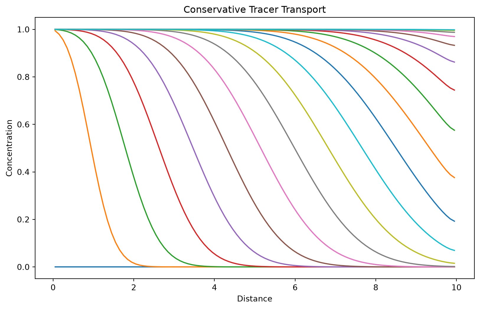
Adding Chemical Reactions
Now let’s extend the model to include a first-order decay reaction:
Step 1: Define the reaction
from reactix import KineticReaction, reaction

@reaction
class FirstOrderDecay(KineticReaction):
    decay_coefficient: jax.Array

    def rate(self, time, state, system):
        # Reaction rate proportional to concentration
        return self.decay_coefficient * state.tracer

    def stoichiometry(self, time, state, system):
        # One mole of tracer consumed per reaction
        return {"tracer": -1}
Step 2: Add reaction to system
# Create reaction instance
decay_reaction = FirstOrderDecay(decay_coefficient=jnp.array(0.1))

# Build system with reactions
reactive_system = System.build(
    porosity=porosity,
    discharge=discharge_rate,
    cells=cells,
    advection=advection,
    dispersion=dispersion,
    species_is_mobile=species_is_mobile,
    bcs=boundary_conditions,
    reactions=[decay_reaction]  # Include the decay reaction
)

# Solve reactive transport
reactive_solution = solver(initial_state, reactive_system)
Multiple Species Example
For systems with multiple interacting species:
# Declare multiple species
Species = declare_species(["substrate", "product"])
species_is_mobile = Species(substrate=True, product=True)

@reaction
class Transformation(KineticReaction):
    rate_constant: jax.Array

    def rate(self, time, state, system):
        return self.rate_constant * state.substrate

    def stoichiometry(self, time, state, system):
        return {
            "substrate": -1,  # Consumed
            "product": 1      # Produced
        }

# Initial state with substrate present
initial_state = Species(
    substrate=jnp.ones(n_cells),  # Initial substrate
    product=jnp.zeros(n_cells)    # No product initially
)
Some Tips
- Units: Be consistent with units across all parameters (length, time, concentration)
- Stability: Use appropriate spatial resolution and solver options (tolerances, type of solver, discretization scheme for the transport terms) for numerical stability.
- Boundary conditions: Ensure boundary conditions are physically reasonable. Not specifying any boundary condition for a species implies a no-flux boundary.
Next Steps
- Explore the Examples for more detailed workflows and use cases
- Check the API Reference for detailed documentation